Stats Tutorial - Instrumental Analysis and Calibration

The Correlation Coefficient:

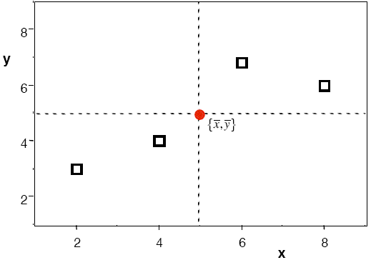
In the first part of this tutorial, we saw how to use the trendline feature in Excel to fit a straight line through calibration data and obtain both the equation of the best-fit straight line and the correlation coefficient, R (often reported as R²). There are in fact various correlation coefficients, but the one we are interested in here is the Pearson or product-moment correlation coefficient. The Pearson R value provides a measure of the degree to which the values of x and y are linearly correlated. We can assess this visually using a scatter plot (Figure 1), in which we also mark the centroid of the data, .

Figure 1 - XY scatter plot showing the centroid of the data

Calculating R:

If x and y were linearly correlated, we would expect all the points to fall on a straight line passing through the centroid. As a result, we would expect all x values to be uniformly distributed about ; similarly, all the y values should be uniformly distributed about . The Pearson R is calculated using the formula:

Note from the equation that R is a function of both the x and y residuals from their respective means. If x and y are perfectly correlated in a linear fashion, we would expect the value of R to be +1 if y increases with increasing x (positive slope), or −1 if y decreases with increasing x (negative slope).

Exercise 1: Calculating R in Excel™

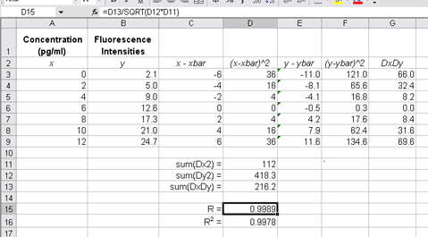
To demonstrate how to calculate this formula in Excel™, we return to our previous example of fluorescence intensity data. Open the relevant Excel™ file from that exercise, and move the chart out of the way if necessary. Then:

1. Set up a spreadsheet with the x_i and y_i values in columns
2. In the adjacent cells, set up expressions for the residuals , , their squares, and their product. For instance, the formula for may look like =B3-AVERAGE(B$2:B$8), depending on the location of your cells in the spreadsheets.
3. Determine the sums of squares and , and the sum of products in Excel and insert these values in the formula for R.
4. To calculate the square root in the denominator, use the SQRT function.
5. Confirm that you obtain the same value of R or R² as reported for the linear trendline fitted earlier.

Solution:

The image below shows one way of setting up the calculation in Excel™. This yields a correlation coefficient R²=0.9978, so the data are reasonably well correlated and can be fitted using a linear equation.

The following equation is an alternate and simpler way to calculate the correlation coefficient. It is left as an exercise for the reader to verify and implement this formula:

More On Calculating R:

A few points to mention regarding the correlation coefficient:

• When calculating manually, it is essential to retain a large number of figures in the numerator and denominator during the calculation, otherwise a misleading value of R may be obtained. Never omit non-significant digits during intermediate steps in the calculation!
• Even a high R value of, say, 0.9991 does not necessarily indicate that the data fits to a straight line. The trendline should always be plotted and inspected visually. R² is more discriminating in this respect, although it no longer indicates the slope of the regression line. This, however, is evident by inspection.
• Any curvature in the data will result in erroneous conclusions about the correlation. R values are only applicable to linear correlations. Nonlinear correlations are possible, but involve a different measure than R, and R values will not necessarily be close to 1.
• The statistical significance of R depends on the number of samples in the data set n, i.e. the number of calibration points used.

Continue with Linear Portions...