Errors, Uncertainty, and Residuals:

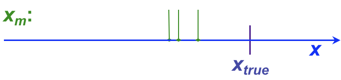
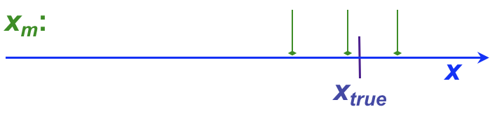
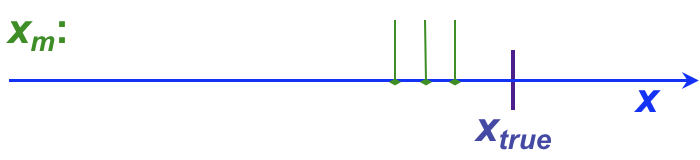
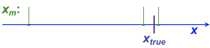
It is not uncommon for analytical chemists to use the terms, “error” and “uncertainty” somewhat interchangeably, although this can cause confusion. This section introduces both terms, as well as providing a more formal introduction to the concept of residuals. Whether error or uncertainty is used, however, the primary aim of such discussion in analytical chemistry is to determine (a) how close a result is to the ‘true’ value (the accuracy) and (b) how well replicate values agree with one another (the precision).

Tips & links:

Skip to Types of Error

Skip to Error & Uncertainty

Skip to Residuals

Types of Error:

In the preceding section, we noted how successive measurements of the same parameter, for the same sample and method, will result in a set of values which vary from the ‘true’ value by differing amounts. In other words, our measurements are subject to error. This is the principal reason why a result based on a single measurement is meaningless in scientific terms. Formally, the error is defined as the result of the measurement minus the true value, (xi − μ). Consequently, errors have both sign and units.

Errors are further categorized in terms of their origin and effect on the measured result:

Systematic errors
are errors that always have the same magnitude and sign, resulting in a bias of the measured values from the true value. An example would be a ruler missing the first 1 mm of its length – it will consistently give lengths that are 1 mm too short. Systematic errors affect the accuracy of the final result, and are also known as determinate errors. The following diagram illustrates the effect of systematic error on a set of replicate measurements (green bars) compared to the true value (blue bar):
depiction of results on a number line showing the effect of systematic error
Random errors
will have different magnitudes and signs, and result in a spread or dispersion of the measured values from the true value. An example would be any electronic measuring device – random electrical noise within its electronic components will cause the reading to fluctuate, even if the signal it is measuring is completely constant. Random errors affect the precision of the final result; they may also affect accuracy if the number of replicates used is too small. Random errors are also knowns as indeterminate errors. The following diagram illustrates the effect of random error on a set of replicate measurements (green bars) compared to the true value (blue bar) both without (upper) and with (lower) the presence of bias:
depiction of results on a number line showing 
						the effect of random error without bias
depiction of results on a number line showing 
						the effect of random error with bias
Gross errors
are errors that are so serious (i.e. large in magnitude) that they cannot be attributed to either systematic or random errors associated with the sample, instrument, or procedure. An example would be writing down a value of 100 when the reading was actually 1.00. If included in calculations, gross errors will tend to affect both accuracy and precision. A single gross error in a set of readings or measurements is termed an outlier. The following diagram illustrates the effect of gross error on a single measurement within a set of replicates (green bars) compared to the true value (blue bar):
depiction of results on a number line showing 
						an extreme outlier in a set of replicate measurements

Back to Introduction

Skip to Error & Uncertainty

Skip to Residuals

Error & Uncertainty:

It should be obvious on reflection that systematic and random errors cannot actually be determined unless the true value, xtrue or μ, is known.

As an example, consider a titration in which the same 25.00 mL pipette is used to dispense portions of the sample for replicate determinations. Due to variations in manufacture, we know that the volume of pure water delivered by the pipette at a specified temperature is ±0.03 mL. In other words, the volume of sample might be 24.98 mL (a systematic error of -0.02 mL) or 25.03 mL (a systematic error of +0.03 mL).

We could in theory determine this error for a specific pipette by calibrating it through weighing replicate volumes dispensed by the pipette, and then converting the mass of pure water to volume. This, however, raises other sources of error:

  • each weight will have its own associated error
  • the operator will not use the pipette in exactly the same way every time, introducing additional error
  • to do the calculation, we need to measure the temperature, which also has an associated error
  • evaporation losses, and changes in temperature and humidity can also contribute to variation in the measured volumes

Clearly, it is unrealistic to try and account for all these errors just to perform every titration. We therefore use an estimate of the error in the volume dispensed by the pipette, which we term the uncertainty. Similarly, any measured value has an associated measurement uncertainty, which is used as an estimate of the range within which the error lies either side of the actual value. Since we cannot easily tell whether the result is above or below the true value, such uncertainties are treated in the same way as random errors.

Back to Introduction

Back to Types of Error

Skip to Residuals

The uncertainty for volumetric glassware is expressed as a manufacturer’s tolerance value, based on batch calibration of the glassware.

A table of common values is available.

Residuals:

Residuals were first introduced in the discussion of variance and standard deviation. The residual is simply the difference between a single observed value and the sample mean, , and has both sign and units. For example, the following table shows individual measurements for the mass of sodium in a can of soup given previously, along with the mean value and residuals:

TrialMass of Na / mgResidual (mg)
1108.6+6.46
2104.2+2.06
396.1-6.04
499.6-2.54
5102.2+0.06
Mean102.1

Residuals can provide a useful comparison between successive individual values within a set of measurements, particularly when presented visually in the form of a residual plot. Such plots can reveal useful information about the quality of the data set, such as whether there is a systematic drift in an instrument under calibration, or if there might be cross-contamination between samples of high and low concentration.

Continue to Probability Distributions...