Stats Tutorial - Instrumental Analysis and Calibration

Dealing with Outliers:

A common problem encountered in instrument calibration is when one or two measurements are clearly ‘off’ – that is, they lie some distance from the regression line when all the other calibration points are close to it. Typically, this is the result of a gross error on the part of the operator, either when preparing the solution or performing the measurement.

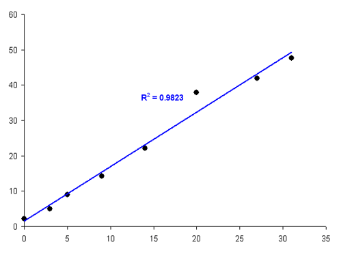
Consider for example the graph below: the value at x_i = 20 is possibly an outlier and skewing the regression line. Can we discard it? A starting point is to calculate the regression residuals and examine them individually. Note that the residual for the suspect point is noticeably different from the others:

Such a point that lies “far away” from the expected value, i.e. has a large regression residual, is called an outlier. Such outliers can easily skew your regression line. However, they can also reveal information about an incomplete regression, or the requirement for more a complex regression model. It is therefore important to know how to deal with such values.

One way of dealing with outliers is to use either weighted linear regression* (in which the standard deviations for replicate determinations of each calibration point are used as “weights” within the analysis), or robust techniques which use median, rather than mean, values. Such methods are beyond the scope of this tutorial, but can be found in the relevant texts. An alternative approach is to make use of statistical tests developed for identifying outliers amongst replicate values, such as Grubb’s test and Dixon’s Quotient (Q) test.

* A recent article has questioned the use of weighted least-squares regression in calibration. See J. Tellinghuisen, Analyst, 2007, 132, 536-543. (DOI: 10.1039/b701696d).

Calibration with Replicate Values:

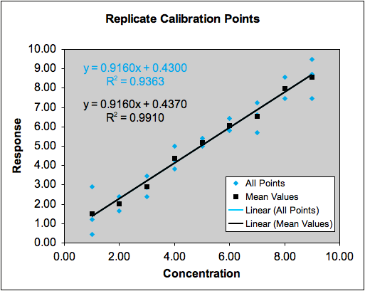
Ideally, each concentration used to construct a calibration curve should be measured at least three times. If one of these values is suspect, it can then be subjected to a statistical test to deterimine if it may be omitted from the data prior to calculating the regression line. Even if the point is not omitted, a form of weighted linear regression can be achieved by entering the replicates for each concentration as separate measurements, rather than as mean values. To some extent, this will reduce the effect of a single outlier among each set of replicates.

To do this in Excel™, you would simply create separate entries in your data table for each replicate of each concentration, then perform your analysis (and plot your calibration curve) using all the values. This has the added benefit that, if you have 5 concentrations measured in triplicate, the number of points in the regression analysis is now n = 5 × 3 = 15, which can reduce the standard errors in the regression, slope, and intercept as well as the uncertainty in any interpolated values.

Note that you may observe a slight difference between the regression line from the result you would get using the mean response for each standard, but the difference is often quite small. The correlation coefficient will, however, be improved using the mean values:

The obvious problem with this approach is that it may simply take too long (or there may not be enough material) to perform replicates for each calibration solution.

Calibration with Single Values:

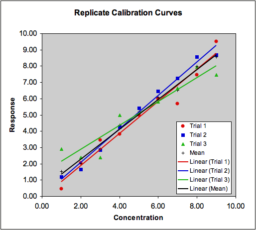
A much more commone situation – especially in techniques such as chromatography, where the run time for a single sample or standard can be significant – is to have only a single value for each calibration point. In this case, you cannot perform an outlier test on the suspect value directly, since your calibration points are supposed to be spread across a range of values. In other words, your highest and lowest concentration standards are, by definition, going to give measurements at either end of the range!

Multiple calibrations with single values compared to the mean of all three trials.

A pragmatic solution is to test the regression residuals for outliers instead. To do this, the residuals are calculated, ranked, and one of two tests applied: Grubb’s test and Dixon’s Quotient (Q) test.

Grubb’s Test:

Grubb’s test can be used to determine whether or not a single outlying value within a set of measurements varies sufficiently from the mean value that it can be statistically classified as not belonging to the same population, and can therefore be omitted from subsequent calculations. As such, it is applied to either the highest or the lowest value in the set; only one value may be omitted from the set on the basis of Grubb’s test.

To perform the test, the mean and standard deviation of all values including the suspect value are calculated. Grubb’s statistic G is then calculated as:

Critical values of G can be calculated for any desired confidence level from the t-statistic, or can be looked up in critical tables. Some selected values at the 95% confidence level are provided; if G > G_critical then the suspect value can be classified as an outlier, and omitted from subsequent calculations.

Dixon’s Quotient (or Q) Test:

Dixon’s Q-test provides a very similar function to Grubb’s test. It has the advantage that the test is simpler to apply, as it does not require calculation of the mean and standard deviation before-hand. A significant disadvantage, however, is that critical values of Q are, in fact, extremely difficult to calculate. A published table of values does exist*, which has made the test quite common in analytical chemistry; the use of Dixon’s Q is, however, deprecated in favour of Grubb’s test.

To perform the Q-test, the measurements are first ranked in order of increasing value. Q is then calculated as the ratio of the difference between the suspect value and its nearest neighbour to the range of the values – hence the name:

Critical values of Q can be looked up in tables at certain confidence levels; if Q > Q_critical then the suspect value can be classified as an outlier, and omitted from subsequent calculations. As with Grubb’s test, only one value from a set of measurements can be omitted in this way which, by definition, will be either x_min or x_max. Dixon’s original paper does treat other situations, such as where the two highest or lowest values are suspect, but calculation of the critical values is even more complex than for a single suspected outlier.

* A corrected table of critical values was published by D. B. Rorabacher in Anal. Chem. 63, 1991, 139-146 (DOI: 10.1021/ac00002a010 ).