Regression Residuals:
The figure below shows an example of a regression line with the
calibration data, centroid (red circle) and y-residuals from
the regression line displayed.
To calculate the regression residuals, we determine the difference between the
measured values (yi) and the values predicted from the actual
concentrations using the regression equation,  (pronounced “y-hat”):
=
bxi + a
yi,res = 
The method of leastsquares (regression of y on x)
effectively tries to minimise these residuals. As
mentioned previously, the residuals provide a convenient means of
checking whether the calibration data is actually linear. To do this,
calculate the regression residuals
for all the points used in the regression analysis, and look for any
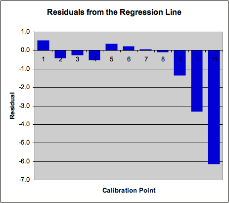
pattern in their magnitude and sign. One easy way to do this is to plot
a bar chart of the residuals. The figure below shows such a plot for the
fluorescence calibration data. Note how the curvature at high concentrations
is clearly visible in the chart:
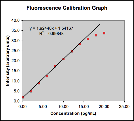
Calibration curve and chart of the residuals
from the regression line for all calibration points; regression line
calculated for the first 9 points in the data set. Notice how the
curvature of the graph at higher concentrations is very evident in
this representation.
Continue to Regression Errors...
 and
and  represent the centroid (mean x & mean y of the
calibration points – use only the values for the linear portion
used when calculating R. The slope and intercept are easily
calculated manually in Excel™ from the table of data used to
generate the plot and calculate R – try this for yourself
using the
represent the centroid (mean x & mean y of the
calibration points – use only the values for the linear portion
used when calculating R. The slope and intercept are easily
calculated manually in Excel™ from the table of data used to
generate the plot and calculate R – try this for yourself
using the