Using Excel’s Functions:
So far, we have been performing regression analysis using only the
simple built-in functions or the
chart trendline options.
However, Excel provides a built-in function called LINEST,
while the Analysis Toolpak provided with some versions includes
a Regression tool. These can be used to simplify regression
calculations, although they each have their own disadvantages, too.
(a) LINEST: You can access LINEST either through the
Insert→Function...
menu item, or by typing the function directly as a formula within a cell.
The function takes up to four arguments: the array of y values,
the array of x values, a value of TRUE if the intercept
is to be calculated explicitly, and a value of TRUE if additional
statistics are to be determined:
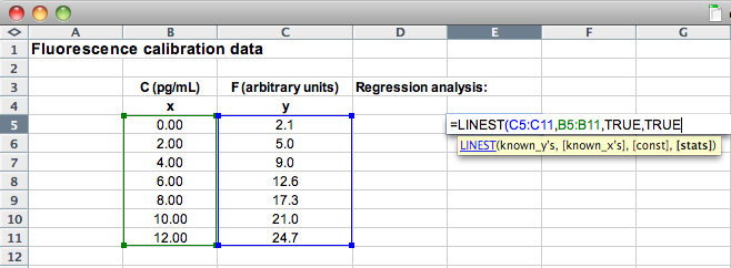
Once you have completed the formula and pressed Enter or return,
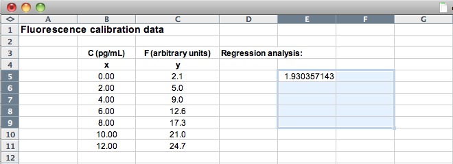
you will see a single value in the cell, which is the slope of the regression line.
To see the rest of the information, you need to tell Excel to expand the results
from LINEST over a range of cells. To do this, first click and drag from
the cell containing your formula so that you end up with a selection consisting of
all the cells in 5 rows and 2 columns:
Now press F2, followed by CTRL+SHIFT+ENTER
(Mac OS: control+u then command+return);
this will expand the results into a table of values:
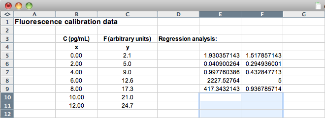
The values obtained in this way are as follows:
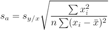
Note that the sum of the last two values (bottom row) is equal to the term
 from the equation for R,
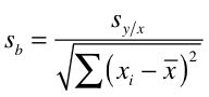
while the sum of the squares of the residuals is used in calculating Sy/x
from the equation for R,
while the sum of the squares of the residuals is used in calculating Sy/x
(b) Regression: Excel 2003 and Excel:Mac 2004 included various
additional utilities that could be added through the Tools menu. If you don’t
see a Data Analysis... item at the bottom of the Tools menu, select the
Add-Ins... item instead. Check the Analysis TookPak item in the dialog
box, then click OK to add this to your installed application.
Once the Data Analysis... item is installed, selecting it will call up a dialog
containing numerous options: select Regression, fill in the fields in the
resulting dialog, and the tool will insert the same regression statistics into your
work sheet.
Continue to Using the Calibration...
 ):
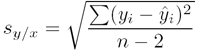
The greater these resdiuals, the greater the uncertainty in where the
true regression line actually lies. The uncertainty in the regression
is therefore calculated in terms of these residuals. Technically, this
is the standard error of the regression, sy/x:
):
The greater these resdiuals, the greater the uncertainty in where the
true regression line actually lies. The uncertainty in the regression
is therefore calculated in terms of these residuals. Technically, this
is the standard error of the regression, sy/x: