Stats Tutorial - Instrumental Analysis and Calibration

Confidence Levels:

We just saw how a series of measurements can follow a normal distribution, such that most of the measurements will be around the mean value, with fewer and fewer measurements occurring the farther away they are from the mean. This can tell us a lot about a dataset. If a certain value is far away from the mean, the chance of randomly getting that value is small. If we take the same measurement numerous times, and keep getting that value, then it is likely that we are measuring a system with a different mean from the one we had previously thought.

So if we get values that are far away from the mean, we can say that there is a small probability that they are part of the same system, but a larger probability that they are part of a different system with a different mean.

Illustrative Example:

Consider the following data set:

2.1, 2.3, 2.6, 2.1, 1.9, 2.2, 1.8, 3.8

The values are centered fairly evenly around 2.3, except for the final value of 3.8. The question is, what is the chance that this large value occurred by random chance, and is it a valid measurement of the system we’re interested in? Or, or is it a spurious result from a different system entirely? We can look at the probability distribution for this set of data, which has a mean of 2.35 and a standard deviation of 0.635. The probability distribution is shown below:

Probability distribution for a system with μ=2.35 and σ=0.635 (solid line), with the experimental values from the above dataset shown as discrete points.

The probability of each value occurring refers to the relative frequency with which each value occurs for a large (n→∞) number of replicate measurements. As you can see, all the measurement values have a fairly high probability of occurring with the exception of 3.8, which would only occur with a probability of less than 0.05, or 5% of the time (1 time in 20).

In other words, if you made many measurements of a system with mean 2.35 and standard deviation 0.635, there is a 5% chance that you would get a result near 3.8. Getting one or two results in the neighbourhood of 3.8 is therefore not completely unlikely, but a large number of results around 3.8 would be highly unlikely.

If were you to observe many values around 3.8, it is much more likely that the system changed while you where working, so that effectively you are measuring a different system to the one you started with. In this case, you could be 95% confident that the value of 3.8 is from a different system. We call this a 95% confidence level, or 95% CL.

Confidence Levels, Limits, and Probabilities:

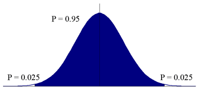
The shaded area of the graph below shows the fraction of all possible values (i.e. the percentage of the total population of values) that fall within 95% of the central mean, μ:

For any given measurement, this fractional area represents a probability of 95% that the resulting value will within a range of possible values either side of the mean as represented by the limits of the shaded area. Notice that there is a small probability of 0.025 (2.5% or 1 chance in 40) that the value will be greater than the upper limit, and the same probability that it will be less than the lower limit; we can also say that there is a probability of 0.05 (5%, or 1 in 20) that the value will not be within the limits either side of the central mean value.

We can calculate these limiting values from the equation of the normal distribution function given earlier. To do this, it is convenient to define a standardized normal variable, z = (x - μ)/σ. Statistical tables provide cumulative values of the NDF as a function of z, from which it is possible to determine that 95% of all possible values lie within the range ±1.96σ on either side of the central mean, μ.

Expressing Confidence Levels:

As we have seen, you can express the level of confidence you have that a measurement is statistically significant (and not the result of an error) in a number of different ways. This can be as a confidence level (e.g. 95% CL), the chances of being correct (19 in 20) or incorrect (1 in 20), or a probability (P = 0.05). You can also talk about a significance level, α, when performing statistical significance tests. α and the CL are related as:

CL = 100 × (1 − α) (%)

If we want to reduce the risk of falsely categorizing a good result as not being significant, we can use a higher confidence level (lower α); to reduce the risk of falsely categorizing a non-significant result as significant, we can use a lower confidence level (higher α).

Most statistical tests discussed in this tutorial ( t-test, F-test, Q-test, etc.) follow a normal curve. If the statistical test shows that a result falls outside the 95% region, you can be 95% certain that the result was not due to random chance, and is a significant result.

These tests will be discussed later in the section on the data evaluation.

Continue to degrees of freedom in statistical calculations...