Stats Tutorial - Instrumental Analysis and Calibration

Calibration Functions:

Every instrument used in chemical analysis can be characterised by a specific calibration function – an equation relating the instrument output signal (S) to the analyte concentration (C). This response function may be linear, logarithmic, exponential, or any other appropriate mathematical form. The exact form of this response function depends on the system being measured and the measurement process itself.

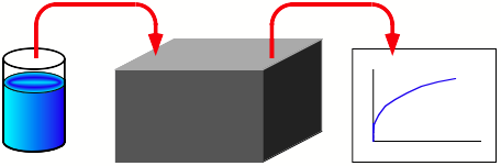
Illustration of the instrument calibration function, S = f(C). Note that the concentration of analyte detected within the instrument may not necessarily be the same as the concentration in the sample, but will be related to it.

While the calibration function may be known theoretically, various factors (such as the specific analyte being measured, interference effects caused by other components of the sample matrix, or random experimental errors) require that we calibrate each instrument for the specific analyte and measurement conditions to be used in a particular experiment.

Types of Function:

As already stated, the calibration curve can take a number of different mathematical forms, depending on the instrument being used. Some examples are listed below:

Type	Equation	Example
Linear (zero intercept)	S=bC	Beer’s Law
Linear (finite intercept)	S=bC+a	Method of standard additions
Logarithmic	S=a+blnC	Nernst Equation
Exponential	S=aebC	Healy's model for immunoassay
Power	S=a+bCn	Kohlrausch’s Law
Polynomial	S=a+bC2+ cC3...	Immunometric assays

The calibration curve is obtained by fitting an appropriate equation to a set of experimental data (calibration data) consisting of the measured responses to known concentrations of analyte. For example, in molecular absorption spectroscopy, we expect the instrument response to follow the Beer-Lambert equation, A = εbC, so we would fit a linear equation with zero intercept to the data.

On the other hand, if we were measuring electrochemical cell potentials (i.e. potentiometry) we would expect the response to be given by the Nernst equation, which is logarithmic in form. We would therefore either fit a logarithmic equation to the calibration data, or linearise the data. This is normally done by calculating log(C), but can also be done by calculating S as 10^E, where E is the measured cell potential.

Deviations from Linearity:

The most common response function encountered in instrumental analytical chemistry is linear, so we require some means of determining and qualifying the best-fit straight line through our calibration data. Before discussing this in detail, however, a word of caution: even when we expect a linear instrument response function, we should not assume that the calibration data must always be linear. In fact, a moment of reflection reveals that we already know that this cannot be true. For example, stray light and polychromatic radiation cause non-linear deviations from Beer's law at higher concentrations; quenching and self-absorption can cause fluorescence intensities to start decreasing with increasing concentration; and column- or detector-overload can cause non-linearities in chromatography.

Proceed to Correlation...